Fitting a Poisson mixture model using EM.

Count data are ubiquitous in science. For example, in biology hightroughput sequencing experiments create huge datasets of gene counts. In this blogpost, I will take a closer look at the Expectation Maximisation (EM) algorithm and use it to derive a Poisson mixture model. To get started, however, we will simulate some data from a Poisson mixture using numpy and scipy.

import numpy as np
import scipy.stats as stats
import matplotlib.pyplot as plt
import seaborn as sns

N = 500
π = np.array([.3, .4, .3])
μ = np.array([30, 100, 150])
Z = stats.multinomial(p=π, n=1).rvs(N) 
_, c = np.where(Z==1)
X = stats.poisson(μ[c]).rvs()  

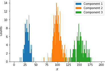
To get a better feeling for these data it is instructive to quickly plot a histogram.

for i in range(len(π)):
    _ = plt.hist(X[c==i], bins=np.arange(200), label=f'Component {i+1}')

plt.legend()
plt.xlabel('$X$')
plt.ylabel('Counts')
sns.despine()
plt.savefig('histogram.png', bbox_inches='tight', pad_inches=0)

The plot nicely illustrates the three clusters in the data centered at roughly 30, 100 and 150. Now, imagine that you had been given these data and your task is to determine the proportion of data belonging to each of the three clusters and their respective cluster centers. In the following, we will first motivate the usage of the EM algorithm, apply it to our problem and finally implement the model in Python.

Defining a Poisson mixture

Let us now formalise the problem. We denote our (synthetic) data with $\mathbf{X}=\{x_1, \dots, x_N\}$ and let $\boldsymbol{\mu}=\{\mu_1,\dots,\mu_K\}$ be the vector representing the cluster means of cluster $k=\{1,\dots, K\}$ . If we are given the cluster $k$ for a data point $x_n$ we can compute its likelihood using

$\begin{aligned} p(x_n|k;\boldsymbol{\mu})= \text{Pois}(x_n; \mu_k). \end{aligned}$

A finite mixture of such Poisson distributions can be expressed as

$\begin{aligned} p(x_n;\boldsymbol{\mu}, \boldsymbol{\pi})= \sum_{k=1}^{K}\pi_k \text{Pois}(x_n; \mu_k) \end{aligned}$

and the likelihood for the whole dataset $\mathbf{X}$ is given by

$p(\mathbf{X};\boldsymbol{\mu}, \boldsymbol{\pi}) = \prod_{n=1}^{N} \sum_{k=1}^{K} \pi_k \text{Pois}(x_n;\mu_k). \tag{1}$

From $(1)$ we can see that it is difficult to optimise the log-likelihood

$\log{p(\mathbf{X};\boldsymbol{\mu}, \boldsymbol{\pi})} = \sum_{n=1}^{N} \log{\sum_{k=1}^{K} \pi_k \text{Pois}(x_n;\mu_k)}, \tag{2}$

as this expression involves the log of sum, making it hard to find close form solutions for the parameters of the model.

The EM algorithm

In the previous section we found that it is infeasible to optimise the marginal log likelihood (Eq. $(2)$). In such cases we can employ the EM algorithm to simplify the optimisation problem. In particular, we will introduce for each data point $x_n$ a corresponding latent variable $\mathbf{z}_n$, and derive the log joint distribution of $x_n$ and $\mathbf{z}_n$ , which is easier to optimise than Eq. $(2)$.

Before we derive the equations to infer the parameters $\boldsymbol{\theta}=\{\boldsymbol{\mu},\boldsymbol{\pi} \}$ of our Poisson mixture, let us quickly recap the EM algorithm (Bishop, 2006).

1. Initialise the parameters of the model $\boldsymbol{\theta}^{\text{old}}$ .
2. E-step: Compute the posterior distribution of the latent variable $p(z_{nk}|x_n;\boldsymbol{\theta}^{\text{old}})$ using the current parameter estimates.

3. M-step: Determine the parameter updates by minimising the expected joint log likelihood under the posterior determined in the E-Step

   $\boldsymbol{\theta}^{\text{new}}=\argmin_{\theta}\mathbb{E}_{z_{nk}\sim p(z_{nk}|x_n;\boldsymbol{\theta}^{\text{old}})}[\log{p(\mathbf{Z},\mathbf{X};\boldsymbol{\theta})}].$

4. Check for convergence by means of the log likelihood or parameter values. If the convergence criterion is not satisfied update

   $\boldsymbol{\theta}^{\text{old}}\leftarrow\boldsymbol{\theta}^{\text{new}}$

   and return to step 2.

The joint log likelihood

The first step involves to determine the joint log likelihood of the model. In finite mixture models, $\mathbf{z}_n=(z_{n1}, \dots, z_{nK})^T$ is a binary $K$-dimensional vector in which a single component equals $1$. Hence, we can write the conditional distribution of $x_n$ given $\mathbf{z}_n$

$p(x_n|\mathbf{z}_n;\boldsymbol{\mu})= \prod_{k=1}^{K} \text{Pois}(x_n; \mu_k)^{z_{nk}}$

and the prior for $\mathbf{z}_n$ as

$p(\mathbf{z}_n; \boldsymbol{\pi})=\prod_{k=1}^{K} \pi_{k}^{z_{nk}}.$

The joint probability distribution (for the complete data) is therefore

$p(\mathbf{X},\mathbf{Z};\boldsymbol{\theta})=\prod_{n=1}^{N} p(x_n|\mathbf{z}_n;\boldsymbol{\mu}) \cdot p(\mathbf{z}_n; \boldsymbol{\pi})=\prod_{n=1}^{N}\prod_{k=1}^{K}(\pi_k\text{Pois}(x_n; \mu_k))^{z_{nk}}$

and the log joint

$\log{p(\mathbf{X},\mathbf{Z};\boldsymbol{\theta})}=\sum_{n=1}^{N}\sum_{k=1}^{K}z_{nk}\{\log{\pi_k}+\log{\text{Pois}(x_n; \mu_k)}\}.\tag{3}$

Comparing Eq. $(2)$ and $(3)$ reveals that in the the latter equation the logarithm distributes over the prior and the conditional distribution. This greatly simplifies the optimisation problem.

Setting up the E-step: The latent posterior distribution

To find the posterior distribution of $z_{nk}$ we make use of Bayes rule

$p(z_{nk}|x_n;\boldsymbol{\theta}^{\text{old}})=\frac{p(z_{nk},x_n;\boldsymbol{\theta}^{\text{old}})}{p(x_n;\boldsymbol{\theta}^{\text{old}})}=\frac{\prod_{k=1}^{K}(\pi^{\text{old}}_k\text{Pois}(x_n; \mu^{\text{old}}_k))^{z_{nk}}}{\sum_z \prod_{j=1}^{K}(\pi^{\text{old}}_j\text{Pois}(x_n; \mu^{\text{old}}_j))^{z_{nj}}}$

which can be simplified by noting $\mathbf{z}_n$ is a binary vector

$p(z_{nk}|x_n;\boldsymbol{\theta}^{\text{old}})=\frac{\pi^{\text{old}}_k\text{Pois}(x_n; \mu^{\text{old}}_k)}{\sum_{j=1}^{K}\pi^{\text{old}}_j\text{Pois}(x_n; \mu^{\text{old}}_j)}.\tag{4}$

Completing the M-step

Now that we have derived the joint log likelihood and the posterior distribution of the latent variables, we can take its expectation

$\mathbb{E}_{z_{nk}\sim p(z_{nk}|x_{n};\boldsymbol{\theta}^{\text{old}})}[\log{p(\mathbf{Z},\mathbf{X};\boldsymbol{\theta})}]=\sum_{n=1}^{N}\sum_{k=1}^{K} \mathbb{E}_{z_{nk}\sim p(z_{nk}|x_{n};\boldsymbol{\theta}^{\text{old}})}[z_{nk}]\{\log{\pi_k}+\log{\text{Pois}(x_n; \mu_k)}\}$

which requires us to calculate

$\mathbb{E}_{z_{nk}\sim p(z_{nk}|x_{n};\boldsymbol{\theta}^{\text{old}})}[z_{nk}]=\sum_{k=1}^K z_{nk} p(z_{nk}|x_n;\boldsymbol{\theta}^{\text{old}})=\frac{\pi^{\text{old}}_k\text{Pois}(x_n; \mu^{\text{old}}_k)}{\sum_{j=1}^{K}\pi^{\text{old}}_j\text{Pois}(x_n; \mu^{\text{old}}_j)}=\gamma(z_{nk}).$

Thus we obtain

$\mathbb{E}_{z_{nk}\sim p(z_{nk}|x_{n};\boldsymbol{\theta}^{\text{old}})}[\log{p(\mathbf{Z},\mathbf{X};\boldsymbol{\theta})}]=\sum_{n=1}^{N}\sum_{k=1}^{K} \gamma(z_{nk}) \{\log{\pi_k}+\log{\text{Pois}(x_n; \mu_k)}\}.\tag{5}$

Finally, we need to compute the derivatives with respect to the model parameters and set them to zero

$\frac{\partial \mathbb{E}_{z_{nk}\sim p(z_{nk}|x_{n};\boldsymbol{\theta}^{\text{old}})}[\log{p(\mathbf{Z},\mathbf{X};\boldsymbol{\theta})}]}{\partial \mu_k}=0\quad\text{and}\quad\frac{\partial \mathbb{E}_{z_{nk}\sim p(z_{nk}|x_{n};\boldsymbol{\theta}^{\text{old}})}[\log{p(\mathbf{Z},\mathbf{X};\boldsymbol{\theta})}]}{\partial \pi_k}=0.$

Solving for $\mu_k$ and $\pi_k$ respectively gives us the following update rules

$\mu_k=\frac{\sum_{n=1}^{N}\gamma(z_{nk})x_n}{\sum_{n=1}^{N}\gamma(z_{nk})}\quad\text{and}\quad\pi_k=\frac{\sum_{n=1}^{N}\gamma(z_{nk})}{N}.\tag{6}$

Note that we have to use Lagrange Multipliers in order to obtain the update rule for $\pi_k$.

Implementing the model

After having done the hard math, the actual implementation of the model is straight forward. The PoissonMixture class takes the as arguments the number of desired clusters $K$ and allows to specifify the initial parameters in the __init__ method. The implementation of the E-Step and and M-Step directly follows from Eq. $(4)$ and $(6)$. Finally, the PoissonMixture model provides a function to compute negative log likelihood¹ of the model as well as a fit method that takes the count data as input.

class PoissonMixture():
    def __init__(self, K=2, π_init=None, μ_init=None, max_iter=10):
        self.K = K
        self.max_iter= max_iter
        
        # initialise parameters
        self.μ_old = (
            np.random.choice(X.squeeze(), K).reshape(1, -1) 
            if μ_init is None else μ_init)
        self.π_old = (
            np.array([1/K for _ in range(K)]).reshape(1, -1) 
            if π_init is None else π_init)
        
    def e_step(self, X):
        γ = stats.poisson(self.μ_old).pmf(X) * self.π_old
        γ /= γ.sum(1, keepdims=True)
        return γ
    
    def m_step(self, X, γ):
        μ_new = (γ * X).sum(0) / γ.sum(0)
        π_new = γ.sum(0) / X.shape[0]
        return μ_new, π_new
    
    def nll(self, X, γ):
        return -(γ * (
            stats.poisson(self.μ_old).logpmf(X) 
            + np.log(self.π_old))).sum()
    
    def fit(self, X):
        
        self.history = {
            'nll': np.zeros(self.max_iter),
            'μ': np.zeros((self.max_iter, self.K)),
            'π': np.zeros((self.max_iter, self.K))
        }
        
        prev_nll = np.inf
        for step in range(self.max_iter):
            γ = self.e_step(X)
            μ_new, π_new = self.m_step(X, γ)
            curr_nll = self.nll(X, γ)
        
            self.history['nll'][step] = curr_nll
            self.history['μ'][step] = self.μ_old
            self.history['π'][step] = self.π_old
            
            Δ_nll = curr_nll - prev_nll 
            print(f'Step {i}: NLL={curr_nll:.2f}, Δ={Δ_nll:.2f}')
            prev_nll = curr_nll
            self.μ_old = μ_new
            self.π_old = π_new

To test our model we instatiate it provide the date via the fit method.

m0 = PoissonMixture(3)
m0.fit(X)
Step 0: NLL=12339.65, Δ=-inf
Step 1: NLL=5619.75, Δ=-6719.90
Step 2: NLL=5249.60, Δ=-370.15
Step 3: NLL=4801.28, Δ=-448.32
Step 4: NLL=3458.16, Δ=-1343.11
Step 5: NLL=2372.49, Δ=-1085.67
Step 6: NLL=2346.74, Δ=-25.75
Step 7: NLL=2345.87, Δ=-0.87
Step 8: NLL=2345.85, Δ=-0.02
Step 9: NLL=2345.85, Δ=0.00

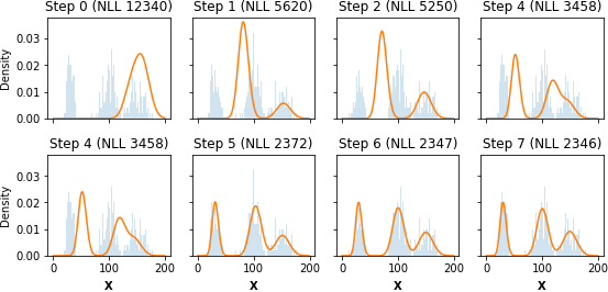
We find that the EM algorithm quickly converges to the optimal solutions, although obviously this implementation is for demonstration purposes only.

Conclusion

In this article we have derived the EM algorithm to fit Poisson mixture models. Further extensions of the model could involve the incorporation of a prior for $\boldsymbol{\mu}$ or $\boldsymbol{\pi}$.