Fully Connected Sigmoid Networks
In this article, I explore how autoregression, typically used in temporal or sequential data, can be applied to images. I framed the problem by treating each pixel as a sequential data point, and modeled its structure using a fully connected sigmoid network. We will see how such a model can be used to model the images of the Caltech Silhouette dataset, which consists of binary (0 or 1) grayscale images.
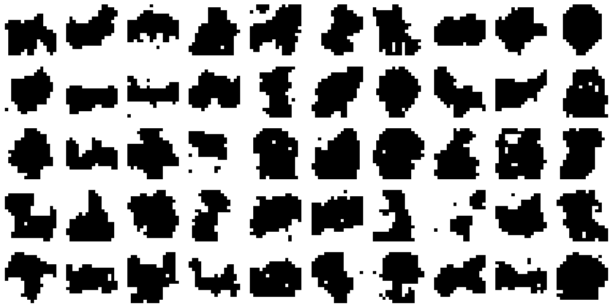
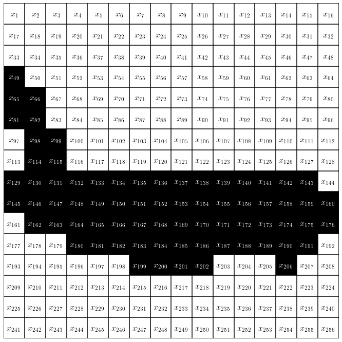
The context of autoregression in terms of temporal data or language is pretty straightforward. Stock prices can rise or fall over time, similarly the order of words in a sentence is not random or independent of each other. But how can we understand autoregression in the context of images ? One possible way to frame images in an autoregression problem is to look one pixel at a time, starting from the top left corner of the image and moving then to the right until we hit the right border and then to continue in the next line. Then we can regard each individual pixel $x_n$ as a data point in a sequence of $n={1,\dots,N}$ data points. In the case of the Caltech Silhouette dataset (Fig. 1), where the data comprises a set of greyscale images, the individual $x_n$ take either the values 0 or 1.
Modeling the state space images
Modeling even simple images, such as those from the Caltech Silhouette dataset, is a hard problem. To see this, consider the large state space of such images. Each pixel can take on either the value 0 or 1 and we have 16 $\times$ 16 of them. This gives us in theory $2^{256}$ possible images. In a generative modelling approach, where the goal is to model the data distribtion over $p_X(x)$, this would require us to assign a probability to each individual realisation of this state space. In other words, specifying the joint distribution over such images requires $2^n-1$ parameters (the minus stems that probability distributions have to sum to 1 and have therefore one degree of freedom less). Certainly this is intractable, nor particularly useful because data contain some inherent structure. In fact, most of the random images you could come up with do not make sense at all (Fig. 2).
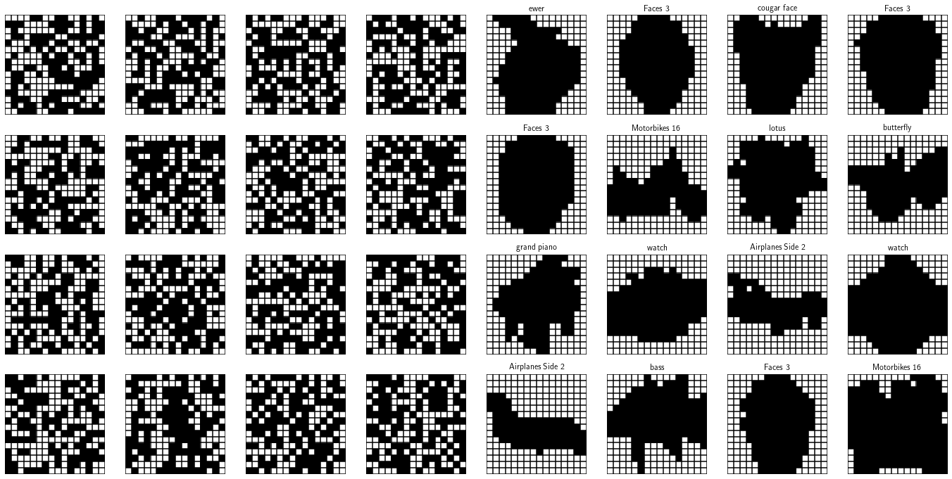
From the images above it becomes clear that there are dependencies in the image. For example if a particular pixel is white, it is more likely that surrounding pixels are white too and vice versa. For this reason, it is intuitive that modelling the joint distribution of an image $p_X(x_1, \dots,x_n)$ is somewhat wasteful if we assume that each $x_n$ is independent
as we clearly neglect the fact that a particular state of a random variable (pixel) is influenced by the surrounding pixels.
Indeed, one way to address this issue is to incorporate structure into the model. The perhaps simplest structure one can perhaps think of is to make each pixel dependent on the pixels before. This is the simplest form of an autoregressive model. Probabilistically this corresponds to saying
A better way - imposing an autoregressive structure
In fully visible belief network we parameterize each of the conditionals on the left hand side using simple logistic or sigmoid models
where the $\mathbf{W}$ and $\mathbf{b}$ denote weight and bias parameters of a linear layer in a neural network1, and $\sigma$ the sigmoid function. It turns out that implementing such a model is relatively easy. To compute the logits2 of the model, we employ simple matrix multiplication but ensure to satisfy the autoregressive structure by masking out some weights in the weight matrix $\mathbf{W}$.
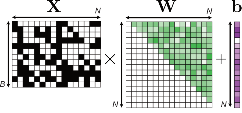
Implementing this model is straightforward in pytorch. The following code block essentially shows how Fig. 3 is implemented in the forward method.
class FVSBN(nn.Module):
    def __init__(self, data_dim, logits=True):
        super().__init__()
        self.data_dim = data_dim
        self.w = nn.Parameter(torch.randn(data_dim, data_dim))
        self.b = nn.Parameter(torch.randn(1, data_dim))

        self.s = nn.Sigmoid()
        self.l = logits

    def forward(self, x):

        original_shape = x.shape
        x = x.view(original_shape[0], -1)
        # input batch x dim * dim
        alpha = torch.tril(self.w, diagonal=-1)
        logits = x @ alpha.T + self.b
        if self.l:
            return logits.view(original_shape)

        return self.s(logits).view(original_shape)
This is essentially all we need to compute all the conditionals per batch. The forward method returns the $B\times N$ matrix of logits. Remember, to train the model we want to maximise the log likelhood of the data. Let $\mathbf{x}^{(j)}$ denote the vector of pixels of an individual image $x_1^{(j)}, \dots, x_N^{(j)}$. Then the log likelihood becomes
and since in this example the pixel values can only take either the values of 0 or 1, we choose a Bernoulli likelihood
which can be easily implemented using the binary_cross_entropy_with_logits loss function.
def loss_fn(inputs, preds):
    loss = F.binary_cross_entropy_with_logits(preds, inputs, reduction="none").sum()
    return loss / inputs.shape[0]
How to sample from the model
Sampling from autoregressive models is somewhat cumbersome as it requires us to sample each random variable $x_1,\dots,x_n$ sequentially, i.e.
where $\bar{x_i}$ represent sampled values from the trained model. To enable sampling from our FCSBNs, we attach a sampling method to the model class.
    def sample(self, num_samples=1, device='cuda'):
        sample = torch.zeros(num_samples, self.data_dim).to(device)
        probs = torch.zeros(num_samples, self.data_dim).to(device)
        i = 0
        for i in range(self.data_dim):
            # print(i, sample)
            p_i = F.sigmoid(sample @ torch.tril(self.w, -1).T[:, i] + self.b[:, i])
            probs[:, i] = p_i
            sample[:, i] = torch.bernoulli(p_i)

        return sample, probs
Results from the Caltech Silhoutte dataset
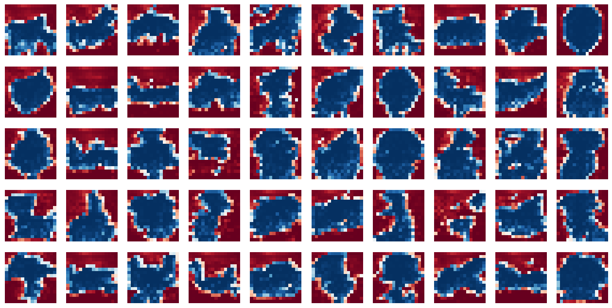
I applied the FCSBN model to the Caltech Silhouette dataset. The following Figures represent some of the sampled images and their corresponding probability maps.
