![]()
Note
In order to run this notebook in Google Colab run the following cells. For best performance make sure that you run the notebook on a GPU instance, i.e. choose from the menu bar Runtime > Change Runtime > Hardware accelerator > GPU.
[3]:
# Install scPCA + dependencies
!pip install --quiet scpca scikit-misc
[2]:
# Download the Kang et. al. dataset
!wget https://www.huber.embl.de/users/harald/scpca/angelidis.h5ad /content/angelidis.h5ad
Analysing the brain cells in light stimulated mice#
In this notebook, we analyse the dataset from Angelidis et. al. in which the authors investigated lung cells of aging mice.
[54]:
import scpca as scp
import numpy as np
import pandas as pd
import matplotlib.pyplot as plt
import scanpy as sc
import seaborn as sns
Data preprocessing#
We begin by importing the dataset with scanpy.
[57]:
data_path = '/content/hrvatin.h5ad'
adata = sc.read_h5ad(data_path)
[58]:
adata
[58]:
AnnData object with n_obs × n_vars = 14745 × 20908
    obs: 'barcode', 'mouse_id', 'age', 'cell_type', 'cell_id'
    uns: 'X_name', 'celltype_column', 'condition_column', 'main_assay'
Examining the obs field of the adata object reveals that the dataset includes two conditions (age column), corresponding to mice aged 3 and 24 months.
[4]:
adata.obs
[4]:
| barcode | mouse_id | age | cell_type | cell_id | |
|---|---|---|---|---|---|
| muc3838:GCACTTTAGAAT | GCACTTTAGAAT | muc3838 | 24m | Ciliated_cells | muc3838:GCACTTTAGAAT |
| muc3838:TCCTGCTCCCTT | TCCTGCTCCCTT | muc3838 | 24m | Ciliated_cells | muc3838:TCCTGCTCCCTT |
| muc3838:TCCTGCTCCCTG | TCCTGCTCCCTG | muc3838 | 24m | Ciliated_cells | muc3838:TCCTGCTCCCTG |
| muc3838:TGCGAGTCTTCT | TGCGAGTCTTCT | muc3838 | 24m | Ciliated_cells | muc3838:TGCGAGTCTTCT |
| muc3838:TCCTGCTCCCTC | TCCTGCTCCCTC | muc3838 | 24m | Ciliated_cells | muc3838:TCCTGCTCCCTC |
| ... | ... | ... | ... | ... | ... |
| muc4657:ATCAAGACAGTG | ATCAAGACAGTG | muc4657 | 3m | Type_2_pneumocytes | muc4657:ATCAAGACAGTG |
| muc4657:GACTGCGCATGG | GACTGCGCATGG | muc4657 | 3m | Ciliated_cells | muc4657:GACTGCGCATGG |
| muc4657:ATGACCGAATGT | ATGACCGAATGT | muc4657 | 3m | Type_2_pneumocytes | muc4657:ATGACCGAATGT |
| muc4657:GTGTTTGGACCG | GTGTTTGGACCG | muc4657 | 3m | Cd4+_T_cells | muc4657:GTGTTTGGACCG |
| muc4657:TGGCCGTGTAGC | TGGCCGTGTAGC | muc4657 | 3m | Goblet_cells | muc4657:TGGCCGTGTAGC |
14745 rows × 5 columns
Before proceeding with the selection of highly variable genes, we filter out low-quality cells and red blood cells, as the latter are not representative of lung cell types.
[5]:
adata = adata[~adata.obs['cell_type'].isin(['low_quality_cells', 'red_blood_cells'])]
[6]:
adata.layers["counts"] = adata.X.copy()
/tmp/ipykernel_657/1517723426.py:1: ImplicitModificationWarning: Setting element `.layers['counts']` of view, initializing view as actual.
  adata.layers["counts"] = adata.X.copy()
[7]:
sc.pp.highly_variable_genes(
    adata,
    n_top_genes=2000,
    flavor="seurat_v3",
    subset=True,
    layer="counts"
)
Factor analysis#
Next, we model the data using scPCA. One strategy is to treat the 3-month condition as the reference and capture gene expression shifts in old mice as deviations from this baseline. This can be specified using the design formula ~ age, similar to how one would define a model in a linear regression framework.
[8]:
m0 = scp.scPCA(
    adata,
    num_factors=10,
    layers_key='counts',
    loadings_formula='age',
    intercept_formula='1',
    seed=8999074
)
[9]:
m0.fit()
  0%|          | 0/5000 [00:00<?, ?it/s]/g/huber/users/voehring/conda/scpca_dev/lib/python3.12/site-packages/scpca/models/scpca.py:68: UserWarning: The use of `x.T` on tensors of dimension other than 2 to reverse their shape is deprecated and it will throw an error in a future release. Consider `x.mT` to transpose batches of matrices or `x.permute(*torch.arange(x.ndim - 1, -1, -1))` to reverse the dimensions of a tensor. (Triggered internally at /pytorch/aten/src/ATen/native/TensorShape.cpp:4413.)
  α_rna = deterministic("α_rna", (1 / α_rna_inv).T)
Epoch: 4990 | lr: 1.00E-02 | ELBO: 2913242 | Δ_10: 43149.50 | Best: 2838556: 100%|██████████| 5000/5000 [02:12<00:00, 37.65it/s]
[10]:
m0.fit(lr=0.001, num_epochs=10000)
Epoch: 14990 | lr: 1.00E-03 | ELBO: 2876858 | Δ_10: 37865.50 | Best: 2809824: 100%|██████████| 10000/10000 [04:08<00:00, 40.29it/s]
Let’s store the result from the factorisation in the adata object.
[11]:
m0.mean_to_anndata(model_key='m0', num_samples=10, num_split=512)
Predicting z for obs 13824-14065.: 100%|██████████| 28/28 [00:02<00:00, 13.78it/s]
If we now take a close look at the adata object we will find that the factors and loadings were added to the obsm and varm fields respectively (X_m0 and W_m0). Meta data related to the model field are stored under adata.uns[{model_key}].
[12]:
adata
[12]:
AnnData object with n_obs × n_vars = 14066 × 2000
    obs: 'barcode', 'mouse_id', 'age', 'cell_type', 'cell_id'
    var: 'highly_variable', 'highly_variable_rank', 'means', 'variances', 'variances_norm'
    uns: 'X_name', 'celltype_column', 'condition_column', 'main_assay', 'hvg', 'm0'
    obsm: 'X_m0'
    varm: 'W_m0'
    layers: 'counts'
Let’s check our factor representation by getting a visual overview using UMAP. We use the UMAP helper function of scpca to accomplish that.
[13]:
scp.tl.umap(adata, 'X_m0')
[14]:
sc.pl.embedding(adata, basis='X_m0_umap', color=['cell_type', 'age'], ncols=1)
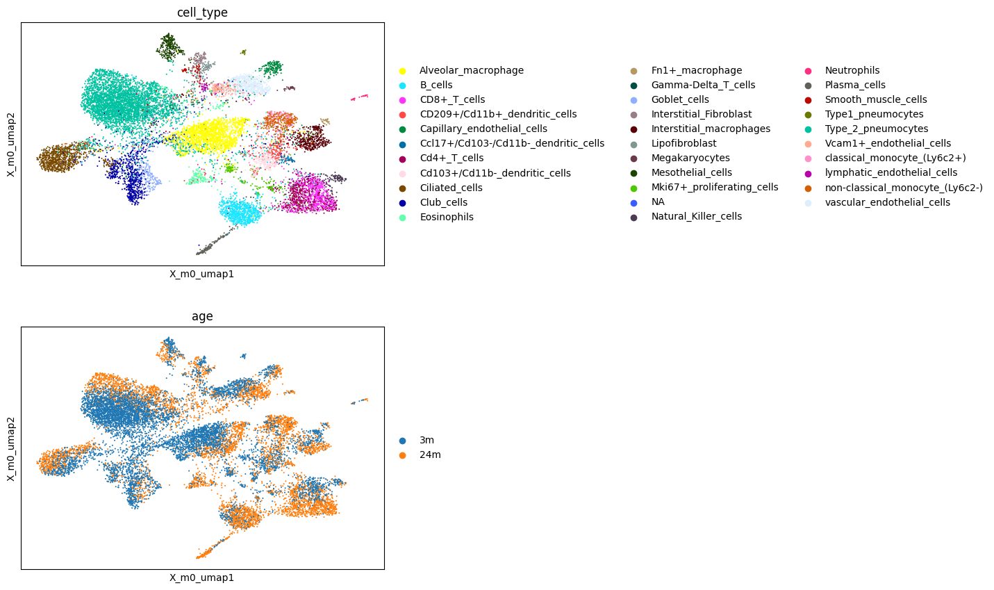
We now try to assess the main factors of the decomposition.
[15]:
scp.pl.factor_embedding(adata, model_key='m0', factor=[0, 1, 2, 3], basis='X_m0_umap', ncols=2)
plt.tight_layout()
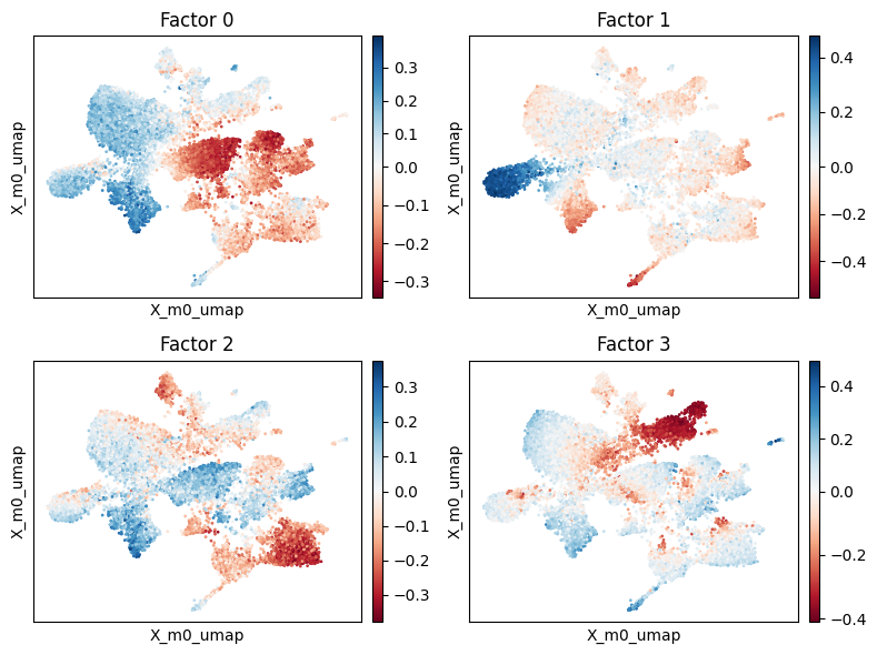
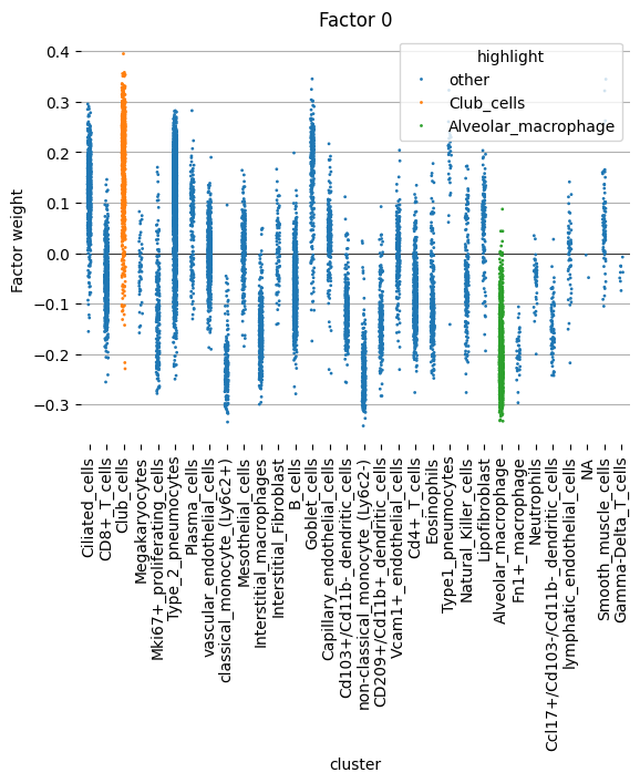
Factor 0#
We begin by examining factor 0 more closely. This factor displays notably negative weights in myeloid cells, including alveolar macrophages and monocytes, and positive weights in club and goblet cells.
[26]:
scp.pl.factor_strip(adata, model_key='m0', factor=[0], cluster_key='cell_type', highlight=['Alveolar_macrophage', 'Club_cells'], s=2)
[26]:
<Axes: title={'center': 'Factor 0'}, xlabel='cluster', ylabel='Factor weight'>
Next we take a close look at the negative loading weights of factor 0 to learn more about the expression patterns in the myeloid cells of this dataset. We can extract those from the adata object using the state_loadings function. Since the factor weights are negative for the myeloid cells, we use the argument lowest=20 and highest=0 to extract the genes with the largest negative loading weights.
[34]:
top_weights_fac0 = scp.tl.state_loadings(adata, 'm0', 'Intercept', 0, highest=0, lowest=20)
[35]:
top_weights_fac0
[35]:
| gene | magnitude | weight | type | state | factor | index | |
|---|---|---|---|---|---|---|---|
| 0 | Abcg1 | 8.844831 | -8.844831 | lowest | 0 | 0 | 73 |
| 1 | Bcl2a1a | 8.854088 | -8.854088 | lowest | 0 | 0 | 162 |
| 2 | Mpeg1 | 9.212790 | -9.212790 | lowest | 0 | 0 | 1053 |
| 3 | Marco | 9.213015 | -9.213015 | lowest | 0 | 0 | 1020 |
| 4 | 1100001G20Rik | 9.315811 | -9.315811 | lowest | 0 | 0 | 0 |
| 5 | Atp6v0d2 | 9.373060 | -9.373060 | lowest | 0 | 0 | 144 |
| 6 | Ltc4s | 9.418015 | -9.418015 | lowest | 0 | 0 | 994 |
| 7 | Fabp1 | 9.497688 | -9.497688 | lowest | 0 | 0 | 542 |
| 8 | Clec4n | 9.505602 | -9.505602 | lowest | 0 | 0 | 368 |
| 9 | Mrc1 | 9.583654 | -9.583654 | lowest | 0 | 0 | 1055 |
| 10 | Ear1 | 9.637006 | -9.637006 | lowest | 0 | 0 | 496 |
| 11 | Bcl2a1d | 9.889424 | -9.889424 | lowest | 0 | 0 | 164 |
| 12 | Clec4a3 | 10.041142 | -10.041142 | lowest | 0 | 0 | 363 |
| 13 | Fcer1g | 10.077384 | -10.077384 | lowest | 0 | 0 | 573 |
| 14 | Tyrobp | 10.141203 | -10.141203 | lowest | 0 | 0 | 1513 |
| 15 | Cybb | 10.273161 | -10.273161 | lowest | 0 | 0 | 435 |
| 16 | Ccl6 | 10.514906 | -10.514906 | lowest | 0 | 0 | 252 |
| 17 | Chi3l3 | 10.604345 | -10.604345 | lowest | 0 | 0 | 340 |
| 18 | Ear2 | 10.699730 | -10.699730 | lowest | 0 | 0 | 498 |
| 19 | Ctss | 10.881914 | -10.881914 | lowest | 0 | 0 | 420 |
As expected the genes are largely associated with myeloid cells, particularly macrophages, and more specifically, alveolar macrophages or monocyte-derived macrophages:
Strong indicators of macrophages / myeloid lineage: Mpeg1, Clec4a3, Clec4n, Fcer1g, Tyrobp, Cybb, Ctss – general myeloid/macrophage markers.
Marco, Mrc1 (CD206) – alveolar macrophage markers; Marco is specific to tissue-resident macrophages like alveolar macrophages.
Chi3l3 (Ym1), Ear1, Ear2, Ccl6 – often upregulated in alternatively activated (M2-like) macrophages in mice.
Bcl2a1a, Bcl2a1d – anti-apoptotic genes, enriched in immune cells including myeloid cells.
Atp6v0d2 – involved in osteoclast/macrophage function.
Ltc4s – leukotriene pathway, expressed in myeloid-derived cells.
Abcg1 – involved in lipid homeostasis, enriched in alveolar macrophages.
Tyrobp – adapter protein for many immune receptors, common in microglia/macrophages.
We next ask the question how the factor 0 changed across conditions. To this end we can compute the loading differences between factor 0 loading weigths between the 24m and 3m condition.
[41]:
_ = scp.pl.loadings_state(adata, 'm0', ['Intercept', 'age[T.24m]'], 0, sign=-1, highest=10, lowest=10, width=4, height=3.5)
plt.tight_layout()
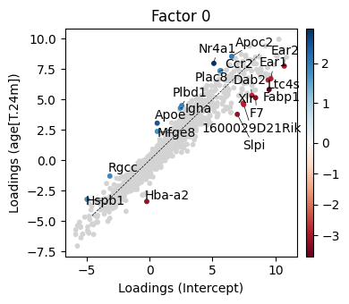
Interestingly we can see here see the downregulation of Ltc4s, Ear1, Ear2 – These are typically expressed in tissue-resident lung macrophages. Their downregulation suggests a shift in macrophage state (e.g., toward a more pro-inflammatory phenotype or loss of identity).
The set of upregulated genes appears to reflect a shift in macrophage state—potentially toward a more inflammatory, monocyte-derived, or activated phenotype, possibly related to aging or stress in the lung environment. This is especially supported by the upregulation of:
Nr4a1: Transcription factor critical for the development of non-classical monocytes; also involved in anti-inflammatory responses and macrophage self-renewal. Upregulation may indicate a monocyte-to-macrophage transition or stress adaptation.
Apoe, Apoc2: Apolipoproteins associated with lipid metabolism and foam-cell–like macrophage states; commonly upregulated in aging, inflammation, or lipid-rich environments (e.g., alveolar space). These are known markers of activated macrophages in chronic inflammation and neurodegeneration, too.
Factor 1#
Next we look at factor 1. Factor 1 exhibits high factor values in Ciliated Cells. Let’s also have a look factor 1s corresponding loading weights.
[31]:
top_weights_fac1 = scp.tl.state_loadings(adata, 'm0', 'Intercept', 1, highest=20)
[33]:
top_weights_fac1.head()
[33]:
| gene | magnitude | weight | type | state | factor | index | |
|---|---|---|---|---|---|---|---|
| 0 | Fam183b | 8.030411 | 8.030411 | highest | 0 | 1 | 554 |
| 1 | 1700016K19Rik | 7.806339 | 7.806339 | highest | 0 | 1 | 15 |
| 2 | Mlf1 | 7.700116 | 7.700116 | highest | 0 | 1 | 1041 |
| 3 | Tmem212 | 7.574149 | 7.574149 | highest | 0 | 1 | 1443 |
| 4 | 1700024G13Rik | 7.569454 | 7.569454 | highest | 0 | 1 | 17 |
[35]:
ax = sns.barplot(data=top_weights_fac1, x='gene', y='weight')
ax.tick_params(axis='x', rotation=90)
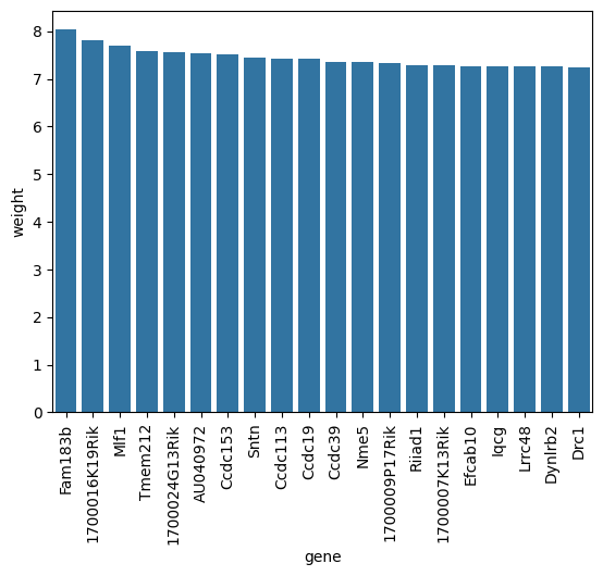
These genes—like CCDC39, Drc1, Dynlrb2, plus several coiled‑coil domain proteins (CCDC113, CCDC153, etc.)—are classic markers of motile cilia structures: they play key roles in axonemal assembly, dynein arm formation, and ciliary motility. For example, CCDC39 is essential for the dynein regulatory complex and inner dynein arms, and DRC1 also has a similar role in ciliary beat regulation.
We next ask the question how the factor 1 changed across conditions. To this end we can compute the loading differences between factor 1 loading weigths from the 24m and 3m condition.
[44]:
_ = scp.pl.loadings_state(adata, 'm0', ['Intercept', 'age[T.24m]'], 1, highest=10, width=4, height=3.5)
plt.tight_layout()
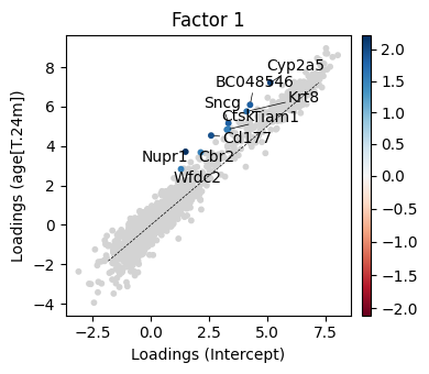
[50]:
top_loading_diff_1 = scp.tl.state_diff(adata, 'm0', ['Intercept', 'age[T.24m]'], 1, highest=20)
These genes, when considered collectively, point to a signature of metabolically active, detoxifying epithelial cells—possibly from liver or lung tissue. They combine:
Detox enzymes and transporters (P450s, Sult1d1, Slc16a11)
Epithelial structural/barrier proteins (Krt8, Cldn3, WFDC2)
Stress response and regulatory factors (Nupr1, Tiam1, Wif1, Dkkl1)
Together these results indicate that scPCAs inferred loading weight differences indicate that ciliated cells shift toward a more metabollically active / stress respond state in old mice.
[ ]: