Note

In order to run this notebook in Google Colab run the following cells. For best performance make sure that you run the notebook on a GPU instance, i.e. choose from the menu bar Runtime > Change Runtime > Hardware accelerator > GPU.

# Install scPCA + dependencies
!pip install --quiet scpca scikit-misc

# Download the Kang et. al. dataset
!wget https://www.huber.embl.de/users/harald/scpca/hrvatin.h5ad /content/hrvatin.h5ad

Analysing the lung cell populations in aging mice

In this notebook, we analyse the dataset from Hrvatin et. al. in which the authors investigated light stimulated brain cells after various time points.

import scpca as scp
import numpy as np
import pandas as pd
import matplotlib.pyplot as plt
import scanpy as sc
import seaborn as sns

Data preprocessing

We begin by importing the dataset with scanpy.

data_path = '/content/hrvatin.h5ad'
adata = sc.read_h5ad(data_path)

adata

AnnData object with n_obs × n_vars = 65539 × 25187
    obs: 'Cell', 'stim', 'sample', 'maintype', 'celltype', 'subtype'
    uns: 'X_name', 'celltype_column', 'condition_column', 'main_assay'

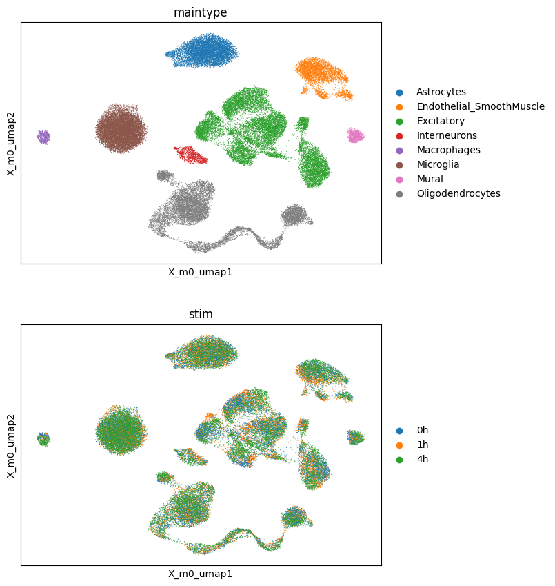
Examining the obs field of the adata object reveals that the dataset includes three different time points (0h, 1h and 4h) in the stim column.

adata.obs

	Cell	stim	sample	maintype	celltype	subtype
x2_35_0_bc0013	x2_35_0_bc0013	0h	B1_1_0h	Excitatory	ExcL4	ExcL4_3
x2_35_0_bc0014	x2_35_0_bc0014	0h	B1_1_0h	Excitatory	ExcL5_3	NA
x2_35_0_bc0016	x2_35_0_bc0016	0h	B1_1_0h	Excitatory	ExcL5_2	NA
x2_35_0_bc0017	x2_35_0_bc0017	0h	B1_1_0h	Excitatory	ExcL6	NA
x2_35_0_bc0018	x2_35_0_bc0018	0h	B1_1_0h	Excitatory	ExcL5_3	NA
...	...	...	...	...	...	...
x2_98_4_2_2_bc2789	x2_98_4_2_2_bc2789	4h	B7_23_4h_B	NA	NA	NA
x2_98_4_2_2_bc2805	x2_98_4_2_2_bc2805	4h	B7_23_4h_B	Microglia	Micro_2	NA
x2_98_4_2_2_bc2823	x2_98_4_2_2_bc2823	4h	B7_23_4h_B	NA	NA	NA
x2_98_4_2_2_bc2857	x2_98_4_2_2_bc2857	4h	B7_23_4h_B	NA	NA	NA
x2_98_4_2_2_bc2997	x2_98_4_2_2_bc2997	4h	B7_23_4h_B	NA	NA	NA

65539 rows × 6 columns

Before proceeding with the selection of highly variable genes, we filter out low-quality (“NA”) cells.

adata = adata[~adata.obs['maintype'].isin(['NA'])]

adata.layers["counts"] = adata.X.copy()

/tmp/ipykernel_3037/1517723426.py:1: ImplicitModificationWarning: Setting element `.layers['counts']` of view, initializing view as actual.
  adata.layers["counts"] = adata.X.copy()

sc.pp.highly_variable_genes(
    adata,
    n_top_genes=2000,
    flavor="seurat_v3",
    subset=True,
    layer="counts"
)

Factor analysis

Next, we model the data using scPCA. One strategy is to designate the 0h condition as the reference and capture gene expression shifts after 1h and 4h as deviations from this baseline. This can be specified using the design formula ~ stim, similar to how one would define a model in a linear regression framework.

m0 = scp.scPCA(
    adata,
    num_factors=10,
    layers_key='counts',
    loadings_formula='stim',
    intercept_formula='1',
    seed=3258035
)

m0.fit()

  0%|          | 0/5000 [00:00<?, ?it/s]/g/huber/users/voehring/conda/scpca_dev/lib/python3.12/site-packages/scpca/models/scpca.py:68: UserWarning: The use of `x.T` on tensors of dimension other than 2 to reverse their shape is deprecated and it will throw an error in a future release. Consider `x.mT` to transpose batches of matrices or `x.permute(*torch.arange(x.ndim - 1, -1, -1))` to reverse the dimensions of a tensor. (Triggered internally at /pytorch/aten/src/ATen/native/TensorShape.cpp:4413.)
  α_rna = deterministic("α_rna", (1 / α_rna_inv).T)
Epoch: 4990 | lr: 1.00E-02 | ELBO: 24579048 | Δ_10: -454472.00 | Best: 23914962: 100%|██████████| 5000/5000 [02:21<00:00, 35.28it/s]

m0.fit(lr=0.001, num_epochs=10000)

Epoch: 14990 | lr: 1.00E-03 | ELBO: 23639794 | Δ_10: -142348.00 | Best: 23275284: 100%|██████████| 10000/10000 [04:38<00:00, 35.87it/s]

Let’s store the result in the adata object.

m0.mean_to_anndata(model_key='m0', num_samples=10, num_split=512)

Predicting z for obs 48128-48265.: 100%|██████████| 95/95 [00:05<00:00, 16.93it/s]

If we now take a close look at the adata object we will find that the factors and loadings were added to the obsm and varm fields respectively (X_m0 and W_m0). Meta data related to the factorisation are stored under adata.uns[{model_key}].

adata

AnnData object with n_obs × n_vars = 48266 × 2000
    obs: 'Cell', 'stim', 'sample', 'maintype', 'celltype', 'subtype'
    var: 'highly_variable', 'highly_variable_rank', 'means', 'variances', 'variances_norm'
    uns: 'X_name', 'celltype_column', 'condition_column', 'main_assay', 'hvg', 'm0'
    obsm: 'X_m0'
    varm: 'W_m0'
    layers: 'counts'

Let’s check our factor representation by getting a visual overview using UMAP. We use the UMAP helper function of scpca to accomplish that.

scp.tl.umap(adata, 'X_m0')

sc.pl.embedding(adata, basis='X_m0_umap', color=['maintype', 'stim'], ncols=1)

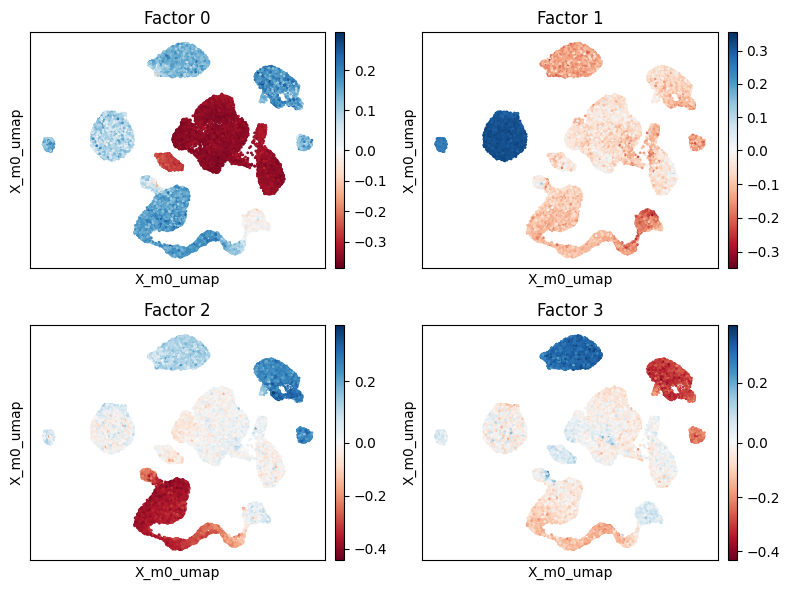
We now try to assess the main factors of the decomposition.

scp.pl.factor_embedding(adata, model_key='m0', factor=[0, 1, 2, 3], basis='X_m0_umap', ncols=2)
plt.tight_layout()

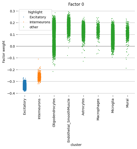
Factor 0

We begin by examining factor 0 more closely. This factor seems to delineate variation between Excitatory/Interneurons and all other cell types.

scp.pl.factor_strip(adata, model_key='m0', factor=[0], cluster_key='maintype', highlight=['Excitatory', 'Interneurons'], s=2)

<Axes: title={'center': 'Factor 0'}, xlabel='cluster', ylabel='Factor weight'>

Next we take a close look at the negative loading weights of factor 0 to learn more about the expression patterns in the myeloid cells of this dataset. We can extract those from the adata object using the state_loadings function. We use the argument lowest=20 and highest=0 to extract the genes with the largest negative weights.

top_weights_fac0 = scp.tl.state_loadings(adata, 'm0', 'Intercept', 0, highest=0, lowest=20)

top_weights_fac0

	gene	magnitude	weight	type	state	factor	index
0	Mal2	10.400877	-10.400877	lowest	0	0	1150
1	Slc6a7	10.412316	-10.412316	lowest	0	0	1699
2	Slc12a5	10.412939	-10.412939	lowest	0	0	1649
3	Trank1	10.452961	-10.452961	lowest	0	0	1889
4	Gabrg2	10.481948	-10.481948	lowest	0	0	729
5	Slc17a7	10.504766	-10.504766	lowest	0	0	1657
6	Tbr1	10.507494	-10.507494	lowest	0	0	1807
7	Adcy1	10.556755	-10.556755	lowest	0	0	116
8	Phf24	10.618876	-10.618876	lowest	0	0	1409
9	Rbfox3	10.658419	-10.658419	lowest	0	0	1531
10	Gpr88	10.676279	-10.676279	lowest	0	0	904
11	Kalrn	10.729308	-10.729308	lowest	0	0	1036
12	Myt1l	10.771517	-10.771517	lowest	0	0	1235
13	Vsnl1	10.859935	-10.859935	lowest	0	0	1954
14	Lamp5	10.900677	-10.900677	lowest	0	0	1088
15	Cck	10.972982	-10.972982	lowest	0	0	325
16	Sncb	11.009183	-11.009183	lowest	0	0	1720
17	Gabra1	11.043131	-11.043131	lowest	0	0	726
18	Nptx1	11.110707	-11.110707	lowest	0	0	1281
19	Sv2b	11.851362	-11.851362	lowest	0	0	1786

Expectedly, we find that these these loadings indicate excitatory neurons.

Gene	Annotation
Slc17a7 (VGLUT1)	Marker of glutamatergic (excitatory) neurons, especially in cortex and hippocampus.
Tbr1	Transcription factor enriched in layer 6 excitatory neurons of the cortex.
Rbfox3 (NeuN)	General neuronal marker, nuclear protein expressed in most mature neurons.
Gabra1, Gabrg2	Encode GABA-A receptor subunits – expressed in both inhibitory and excitatory neurons (receptive to GABA).
Cck, Lamp5	Typically associated with interneurons, but also found in specific excitatory subtypes, particularly in superficial cortical layers.
Slc12a5 (KCC2)	Potassium-chloride transporter critical for neuronal chloride homeostasis – enriched in mature excitatory neurons.
Slc6a7	High-affinity L-proline transporter, enriched in glutamatergic neurons, possibly in layer 5/6.
Mal2, Kalrn, Adcy1, Phf24, Trank1, Gpr88, Sncb, Myt1l, Vsnl1, Nptx1, Sv2b	Involved in synaptic function, neuronal maturation, and plasticity. Most are enriched in excitatory neurons of the cortex.

Next, we would like to understand how the factor 0 weights change across the condtitions. We provide the scp.pl.loadings_scatter function to visualise the loading weights across several condtions. This function requires us to specify the genes we want to visualise. To find interesting genes we focus on the genes with largest loading state differences between the 0h and 1h condition.

loading_diff0 = scp.tl.state_diff(adata, model_key='m0', states=['Intercept', 'stim[T.1h]'], factor=0, sign=-1)

scp.pl.loadings_scatter(adata, 'm0', ['Intercept', 'stim[T.1h]', 'stim[T.4h]'], 0, sign=-1, var_names=loading_diff0.gene.tolist(), show_labels=1)

<Axes: title={'center': 'Factor 0'}, xlabel='State', ylabel='Loading weight'>

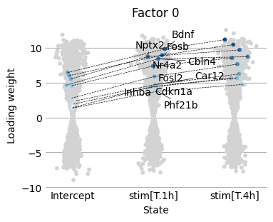
We find that this gene set is enriched for neuronal immediate early genes (IEGs) and activity-induced transcription factors.

Gene	Function / Annotation
Fosb, Fosl2	Core immediate early genes (IEGs); rapidly induced by neuronal activity; components of the AP-1 transcription factor complex.
Egr2, Egr4	Early growth response transcription factors; induced by neuronal depolarization and activity.
Nr4a2	Nuclear receptor involved in dopaminergic neuron function, plasticity, and survival.
Gadd45b	Activity-dependent gene involved in DNA demethylation and neuroplasticity.
Tnfaip6	Induced by inflammation and neuronal stimulation; involved in extracellular matrix remodeling.
Bdnf	Brain-derived neurotrophic factor; crucial for synaptic plasticity, learning, and memory.
Pim1	Activity-induced serine/threonine kinase, regulates cell survival in neurons.
Nptx2	Neuronal pentraxin, secreted protein involved in synapse remodeling and homeostatic plasticity.

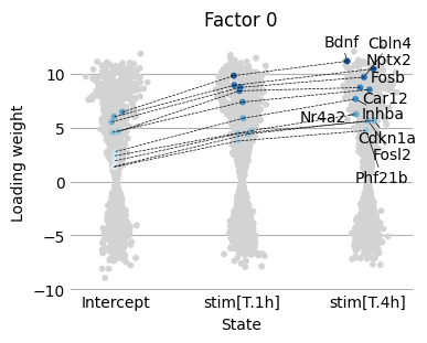
Likewise we can try to elucdiate gene expression shifts between reference (baseline) and 4h condition.

loading_diff0 = scp.tl.state_diff(adata, model_key='m0', states=['Intercept', 'stim[T.4h]'], factor=0, sign=-1)

scp.pl.loadings_scatter(adata, 'm0', ['Intercept', 'stim[T.1h]', 'stim[T.4h]'], 0, sign=-1, var_names=loading_diff0.gene.tolist(), show_labels=2)

<Axes: title={'center': 'Factor 0'}, xlabel='State', ylabel='Loading weight'>